Options
On the Options tab of the Point Cloud Modelling form, set the parameters and define the surface area for the interpolation.
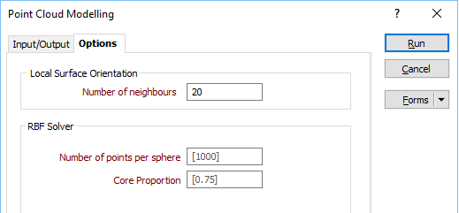
Local Surface Orientation
Number of Neighbours
This parameter is used to control local orientation of the modelled surface. In particular it is used to define the direction perpendicular to the surface. In other words it determines what is the “top” and “bottom” of the surface at any location. A minimum of 4 points are required for this calculation.
Note: Try starting between 6 (sparse) and 20 (dense).
RBF Solver
In most cases it is impractical to create a single model using all the points in the data set. Instead the data set can be divided into overlapping regions. These regions are defined by the direction of propagation of spheres across the input data:
The Number of points per sphere is the number of points you want to look at per sphere. The radius of each sphere will therefore depend on the concentration and the distribution of the points in the input data.
Core Proportion is a number between 0 and 1. This value reduces the radius of the larger sphere to a smaller one as the spheres are propagated.
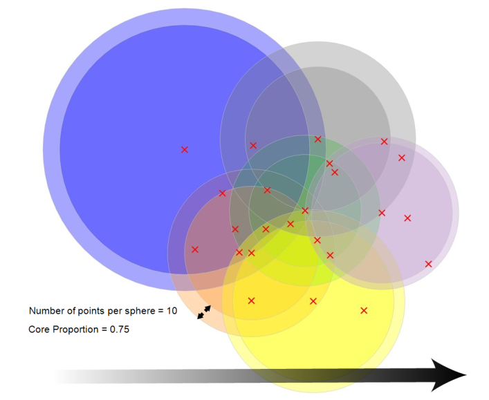
For sparse data, a Core Proportion of [0.75] is the default. This defines a 25% overlap of the points in adjoining spheres. The lower the value, the higher the overlap between the spheres.
Weighting
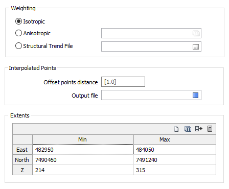
Select a Weighting option:
- When you select an Isotropic search, there is no preferred direction.
- When you select an Anisotropic search, you enter a preferred direction, as well as specify the weighting in that direction.
- When you select Structural Trend File, a data search weighting is derived from the direction of anisotropy defined in a (*.mmstf) Structural Trend File, which is an output of the Implicit Modelling | Create Structural Trend function.
Double-click to load an existing form set. Alternatively, right-click in the Anisotropic input box to open a form where you can define the shape and direction of the search ellipsoid.
The ability to apply a weighting based on the orientation of a data search ellipsoid is a useful option. Although it references the same set of parameters used to define a data search for block modelling, only a few of the values are utilised by implicit modelling.
For example, only the factors and rotation associated with the orientation axes are used – the radius is ignored and will be greyed out. If you consider that there is a greater correlation in a particular direction, then select Ellipsoidal, and set appropriate factor, azimuth, plunge and rotation values.
This effectively accounts for any anisotropy. Interpolation weights can be adjusted accordingly; data points located along the major semi-axis will receive a higher weighting than those located along the minor semi-axis, for similar distances from the prediction location.
Interpolated Points
As part of the modelling process, the RBF function will generate interpolated points in the (+/-) directions of the normal.
However, when interpolating off-surface points, you should ensure that those points do not intersect other parts of the surface. Points must be interpolated an appropriate distance along the normals so that the closest surface point to each interpolated point is the surface point it was generated from.
Offset points distance
Enter an appropriate distance value which is consistent with the surface data.
Output file
Double-click (or click on the Select icon) to select the name of the file where the interpolated points will be written.
Extents
Define the area of interpolation:
East, North and Z fields
Specify the Minimum and Maximum extents of the surface in the East, North and Z directions.
You can use the buttons on the grid list toolbar (or use the right-click menu) to Manage the rows in the list.